Examples

Tinyopt C Examples

The examples use the C API described in the C API guide. They link against the library built by pixi run build-c-library (build-c-library/), for instance:

pixi run build-c-library
cc examples/c/quadratic.c -Iinclude -Ibuild-c-library/generated/include \
   -Lbuild-c-library -ltinyopt_c -Wl,-rpath,"$PWD/build-c-library" -o quadratic && ./quadratic

With -DTINYOPT_BUILD_EXAMPLES=ON CMake also builds them (as tinyopt_example_c_*).

Example	Evaluation mode	Problem
quadratic.c	TINYOPT_EVAL_RESIDUALS	Smallest dynamic-size fit, with a hand-written Jacobian.
fixed_circle_fit.c	TINYOPT_EVAL_RESIDUALS	Circle fit with fixed-size 3 parameters (tinyopt_optimize3).
dynamic_cost.c	TINYOPT_EVAL_COST_ONLY	Scalar objective only, the gradient is estimated numerically.
manual_gradient.c	TINYOPT_EVAL_GRADIENT	Gradient descent on a hand-accumulated cost and gradient.
manual_hessian.c	TINYOPT_EVAL_HESSIAN	Hand-accumulated cost, gradient and Hessian.
sparse_hessian.c	sparse Hessian	Tridiagonal signal smoothing with CHOLMOD (needs TINYOPT_ENABLE_SUITESPARSE=ON).

Tinyopt C++ Examples

Build all examples with pixi run build-examples. The standalone executables are written under build-examples/examples/cpp/; run any target there to see its estimated parameters and solver status. The C++ API is described in the API doc and the tutorial.

Domain	Example	Solver	Problem
Finance	finance.cpp	L-BFGS	Long-only mean-variance portfolio fit
Computer vision	computer_vision.cpp	Gauss-Newton	Pinhole camera calibration
Biology	biology.cpp	BFGS	Logistic population-growth fit
Astronomy	astronomy.cpp	Levenberg-Marquardt	One-dimensional astrometry with parallax
Physics	physics.cpp	Dogleg	Damped oscillator parameter fit
Robotics	robotics.cpp	Gradient descent	2D landmark-based translation estimate
Signal processing	signal_processing.cpp	Conjugate gradient	Sinusoid amplitude and offset fit

Each program is standalone and uses only Tinyopt and the C++ standard library.

Tinyopt WebAssembly / JavaScript Example

Tinyopt’s C API compiled to WebAssembly with Emscripten and driven directly from JavaScript, no glue code: optimizer.js writes the C structs into the module memory and passes JavaScript functions as the C callbacks.

pixi run build-wasm      # build-wasm/wasm-example: tinyopt.mjs + tinyopt.wasm + the page
pixi run test-wasm       # headless check of the module with Node
pixi run wasm-example    # serve it, then open http://localhost:8000

build-wasm cross-compiles the C library into its own build-wasm/ directory (the native build-c-library/ cannot be linked into WebAssembly); it only builds double precision and the 2D fixed size, so it is fast. It needs Emscripten, provided by the wasm pixi environment, and -DTINYOPT_BUILD_WASM=ON when using CMake directly. The page loads three.js from a CDN.

The JS layer exposes a small wrapper object that hides the raw wasm memory writes behind a plain options object and a minimize(problem, start, options) entry point; the example still calls the low-level C ABI underneath, but app code does not need to fight the HEAP32/HEAPF64 layout.

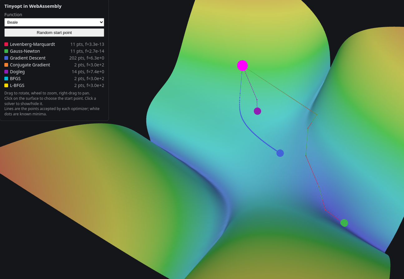
index.html / main.js: optimizer trajectories on 3D cost surfaces

The demo starts with a few beginner-friendly problems (quadratic, linear system, offset plane) and then moves into the classical 2D least-squares cases (Rosenbrock, Himmelblau, Beale, Booth, Freudenstein-Roth). They are solved by Levenberg-Marquardt, Gauss-Newton, Gradient Descent, Conjugate Gradient, Dogleg, BFGS and L-BFGS. The cost is drawn in 3D (log-scaled height).

• Pick the function in the menu, rotate/zoom/pan with the mouse.

• A random start point is used; “Random start point” draws another one.

• Click on the surface to choose the start point.

• Each optimizer has its own color and its trajectory is drawn; click a legend entry to hide it. White dots are the known minima.

Trajectories come from options.step_callback (see the C API guide), which reports every step added to the parameters and every roll-back of a rejected step.

Files

File	Role
problems.js	The five problems: residuals, Jacobians, domains, known minima.
optimizer.js	createOptimizer(): wasm32 struct layout, callbacks, minimize() returning the trajectory.
main.js, index.html	three.js scene and UI.
test.mjs	Node test: Jacobian check, every solver on every problem, layout check against the C defaults.

Residual based solvers (LM, Gauss-Newton, Dogleg) use TINYOPT_EVAL_RESIDUALS; the others (gradient descent, conjugate gradient, BFGS, L-BFGS) use TINYOPT_EVAL_GRADIENT with cost 0.5 * |r|^2 and gradient J^T r. Undamped Gauss-Newton often rejects its first step on these non-linear problems, which is visible as a trajectory reduced to the start point.